return to the trenches
thank you marty, jush, oxmer, colman, and fleetwood for review
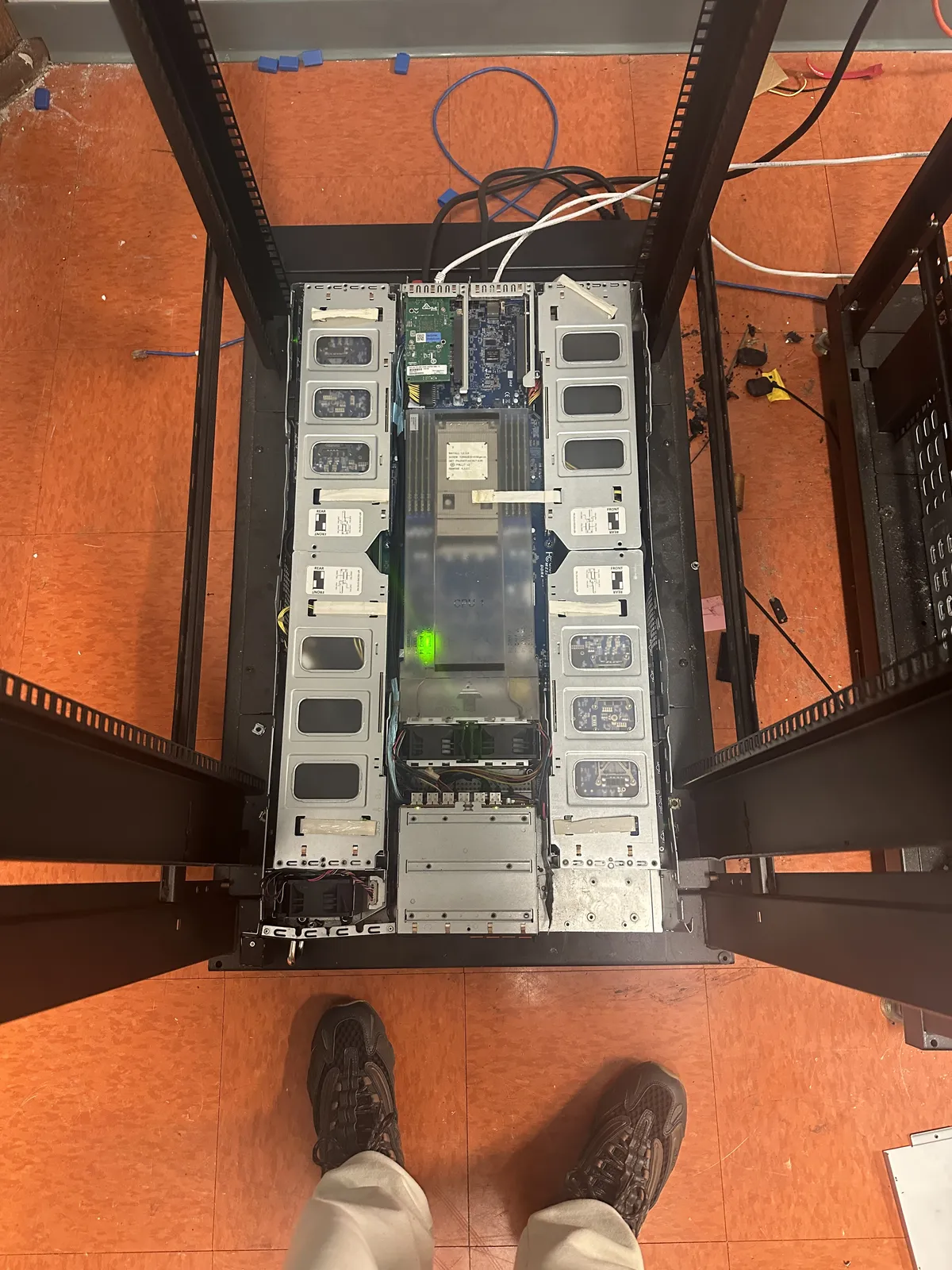
howard is my tenstorrent dev box - 4 N300 cards, 8 wormhole chips, 512 tensix cores, 96gb of gddr6, and an amd epyc to babysit it all. he'd been sitting idle for months. then jim keller appeared in my dream and scolded me for wasting resources. so i'm back in the metal trenches.
the setup
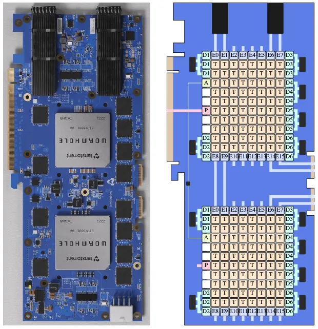
4 N300 cards (8 wormhole b0 chips) in an AMD EPYC 7282 host with 257gb ram. each chip has 64 tensix cores enabled and 12gb gddr6, so up to 512 cores and 96gb total.
the cards form two isolated 2x2 meshes, each wired internally with 100gbe links:
Mesh A (chips 0,1,4,5)      Mesh B (chips 2,3,6,7)
======================      ======================

┌───────┐ 100G ┌───────┐    ┌───────┐ 100G ┌───────┐
│Chip 0 │◄────►│Chip 1 │    │Chip 2 │◄────►│Chip 3 │
│(PCIe) │      │(PCIe) │    │(PCIe) │      │(PCIe) │
└───┬───┘      └───┬───┘    └───┬───┘      └───┬───┘
   100G           100G         100G           100G
┌───┴───┐      ┌───┴───┐    ┌───┴───┐      ┌───┴───┐
│Chip 4 │◄────►│Chip 5 │    │Chip 6 │◄────►│Chip 7 │
│Remote │ 100G │Remote │    │Remote │ 100G │Remote │
└───────┘      └───────┘    └───────┘      └───────┘
tenstorrent's ttnn library gives you the ops, but you're on your own for autograd unless you are using tt-train. i built four autograd implementations, scaled up to gpt-2, then tried to squeeze parallelism out of the hardware. this post covers all of it.
part 1: building an autograd engine
the benchmark
i tested on a 2-layer mlp:
input [1024, 512]
    ↓
linear (512 → 512) + relu
    ↓
linear (512 → 512)
    ↓
mse loss → backward → sgd update
about 525k parameters, 24 ttnn ops per training step (forward, backward, and weight update - not counting host↔device transfers which happen once at setup). all tensors are bf16 in 32x32 tile format (dims must be multiples of 32; my shapes are clean so no padding overhead).
cpu baseline is pytorch 2.2.1 on the epyc (32 cores, fp32). note: this isn't apples-to-apples precision - bf16 mse isn't supported on cpu, so the comparison is "what i can actually run today" rather than equivalent math.
approach 0: python dynamic autograd
started with the obvious - a pytorch-style api on ttnn's python bindings (py/engine.py):
class Tensor:
  def __init__(
      self, data, _children=(),
      _op="", requires_grad=False, device=None):
    # handle both torch and ttnn tensors
    is_ttnn = (hasattr(data, 'shape')
               and not hasattr(data, 'storage'))
    if is_ttnn:
      self.tt = data
    else:
      self.tt = ttnn.from_torch(
        data, device=device,
        layout=ttnn.TILE_LAYOUT)
    self.grad = None
    self.requires_grad = requires_grad
    self._backward = lambda: None
    self._prev = set(_children)

  def __matmul__(self, other):
    out = Tensor(
      ttnn.matmul(self.tt, other.tt),
      (self, other), "matmul")
    def _backward():
      if self.requires_grad:
        g = ttnn.matmul(
          out.grad, other.tt, transpose_b=True)
        self._add_grad(g)
      if other.requires_grad:
        g = ttnn.matmul(
          self.tt, out.grad, transpose_a=True)
        other._add_grad(g)
    out._backward = _backward
    return out
works fine for prototyping. the problem is python overhead - object allocation, function calls, the gil. the ttnn ops are fast, but the python glue adds up.
result: 9.506 ms/iter (0.66x pytorch cpu - actually slower)
wrapping fast accelerator ops in python made it slower than cpu. not great.
approach 1: c++ dynamic autograd
same design, just in c++ (autograd/dynamic/autograd.hpp):
struct Value {
  tt::tt_metal::Tensor data;
  std::optional<tt::tt_metal::Tensor> grad;
  bool requires_grad = false;
  std::function<void()> backward_fn;
  std::vector<std::shared_ptr<Value>> parents;
};
operations create new values and capture backward functions (autograd/dynamic/ops.hpp):
ValuePtr matmul(ValuePtr a, ValuePtr b) {
  auto out = std::make_shared<Value>(
    ttnn::matmul(a->data, b->data));
  out->parents = {a, b};
  out->backward_fn = [a, b, out]() {
    if (a->requires_grad) {
      auto g = ttnn::matmul(
        out->grad.value(), b->data, false, true);
      a->accumulate_grad(g);
    }
    if (b->requires_grad) {
      auto g = ttnn::matmul(
        a->data, out->grad.value(), true, false);
      b->accumulate_grad(g);
    }
  };
  return out;
}
still has per-iteration overhead: host allocations (new shared_ptrs, closures, vectors for topo sort) plus device buffer allocations for each op output. but removing python from the loop lets the wormhole shine.
result: 0.984 ms/iter (6.34x faster than pytorch cpu)
just removing python overhead let the accelerator do its job.
approach 2: static autograd
key insight: if the network architecture doesn't change, why rebuild the graph every iteration?
static autograd pre-allocates the graph's long-lived buffers (activations, params, grads), eliminates per-iteration zeros_like calls, and sets us up to reuse outputs via trace. note: individual ttnn ops still allocate device buffers for their outputs unless you pass output_tensor - the real win comes when combined with tracing (autograd/static/value.hpp):
struct Value {
  // pointer to pre-allocated buffer
  Tensor* data;
  // pointer to gradient buffer
  Tensor* grad;
  bool requires_grad;
  bool grad_initialized = false;
  std::function<void()> backward_fn;
  std::vector<Value*> parents;
};

struct Graph {
  std::vector<std::unique_ptr<Value>> nodes;
  // built once, reused
  std::vector<Value*> topo_order;
  Value* root = nullptr;

  void zero_grad() {
    for (auto& n : nodes)
      // no alloc, just reset flag
      n->grad_initialized = false;
  }
};
the trick for gradient accumulation - track whether it's the first write:
void accumulate_grad(const Tensor& g) {
  if (!grad) return;
  if (!grad_initialized) {
    // first write: overwrite
    *grad = g;
    grad_initialized = true;
  } else {
    // subsequent: accumulate
    *grad = ttnn::add(*grad, g);
  }
}
this eliminates the zeros_like() device allocation every backward pass - the first write just overwrites whatever garbage is in the buffer.
result: 0.673 ms/iter (9.27x faster than pytorch cpu)
the remaining overhead is still significant: each ttnn op allocates new output buffers. that's where tracing comes in.
approach 3: static autograd + trace api
ttnn has a trace api that records operations and replays them without host-side overhead (this is trace capture/replay, not the tracing/visualization tooling) (autograd/traced/trace.hpp):
trace_id = ttnn::begin_trace_capture(device);
model.train_step();  // operations recorded
ttnn::end_trace_capture(device, trace_id);

// later: replay without host dispatch overhead
ttnn::execute_trace(device, trace_id);
because static autograd uses fixed buffers and a persistent graph, it works perfectly with trace capture. the trace records all device buffer allocations and op dispatches once, then replays them with minimal host involvement.
result: 0.563 ms/iter (11.08x faster than pytorch cpu)
mlp results
(bench/autograd/bench_mlp.cpp)
| method | ms/iter | vs torch cpu |
|---|---|---|
| pytorch cpu (fp32) | 6.237 | 1.00x |
| ttnn python dynamic | 9.506 | 0.66x |
| ttnn c++ dynamic | 0.984 | 6.34x |
| ttnn c++ static (persistent) | 0.673 | 9.27x |
| ttnn c++ static + trace | 0.563 | 11.08x |
trace is especially powerful for small shapes where dispatch overhead dominates (bench/autograd/bench_shape_sweep.cpp):
| batch | dim | c++ dynamic | static+trace | speedup |
|---|---|---|---|---|
| 256 | 256 | 1.36 ms | 0.17 ms | 8.1x |
| 256 | 2048 | 1.79 ms | 1.37 ms | 1.3x |
| 2048 | 2048 | 4.12 ms | 3.31 ms | 1.2x |
| 4096 | 2048 | 7.68 ms | 6.43 ms | 1.2x |
at large shapes, dispatch overhead becomes negligible and the implementations converge. this foreshadows what happens at gpt-2 scale.
benchmark notes: all runs on a single wormhole ASIC (64 tensix cores). transfers not included in timing - data is resident on device. bf16 on wormhole vs fp32 on cpu means the speedup ratios reflect practical performance, not equivalent FLOPs.
part 2: scaling to gpt-2
adding embeddings
the mlp benchmark was useful for iteration, but real models need embeddings. ttml (tenstorrent's reference ML library) has a nano_gpt implementation with:
- token embedding [vocab=256, dim=384]
- positional embedding [seq=256, dim=384]
- 6 transformer blocks
- output projection [dim=384, vocab=256]
i added embeddings to match. embedding weights use ROW_MAJOR layout (ttnn requires this for the lookup), while everything else stays in TILE_LAYOUT for efficient matmuls (autograd/traced/nn.hpp):
struct TracedEmbedding {
  // [vocab_size, dim] ROW_MAJOR
  Tensor weight;
  // gradient buffer
  Tensor d_weight;

  void forward(
      const Tensor& indices,
      Tensor& out) {
    out = ttnn::embedding(
      indices, weight,
      std::nullopt, ttnn::TILE_LAYOUT);
  }

  void backward(
      const Tensor& indices,
      const Tensor& d_out) {
    // embedding_bw expects [1, 1, batch*seq, dim]
    auto d_out_reshaped = ttnn::reshape(
      d_out, {1, 1, batch*seq, dim});
    d_weight = ttnn::embedding_bw(
      indices, weight, d_out_reshaped);
  }
};
apples-to-apples comparison
with identical architectures, here's the fair comparison (bench/autograd/bench_gpt2_full.cpp):
| implementation | time (ms) | speedup |
|---|---|---|
| ttml nano_gpt | 510.0 | 1.00x |
| static+trace (ours) | 323.0 | 1.58x |
1.58x faster with the same architecture, same ops, same backward formulas. the gap comes from eliminating per-iteration overhead: pre-allocated buffers and the overwrite-on-first-write trick mean zero dynamic allocation during training. ttml rebuilds its autograd graph every iteration.
when tracing stops helping
here's the twist: tracing gave us 8x on the small mlp. but on gpt-2? (bench/autograd/bench_gpt2_trace.cpp)
| mode | total (ms) | per-layer (ms) | speedup |
|---|---|---|---|
| static | 323.05 | 53.84 | 1.00x |
| traced | 323.09 | 53.85 | 1.0x |
tracing does nothing for the full gpt-2. why?
the model is compute-bound, not dispatch-bound:
- each matmul is [32, 256] × [384, 256] or larger
- attention computes [32, 6, 256, 256] score matrices (batch, heads, seq, seq)
- embedding lookup touches [256, 384] weight matrices
at these sizes, tensor computation dominates. the ~0.1ms dispatch overhead per op is negligible when each op takes 50+ ms.
the pattern:
| model | dispatch-bound? | trace speedup |
|---|---|---|
| mlp (256×256) | yes | 8x |
| mlp (2048×2048) | no | 1.2x |
| full gpt-2 | no | 1.0x |
gradient correctness
"but do your gradients actually match?" fair question. i verified against pytorch (verify/compare_grads.py):
| operation | max diff | status |
|---|---|---|
| embedding forward | 0.00002 | ✓ |
| linear forward | 0.00027 | ✓ |
| linear d_input | 0.00033 | ✓ |
| linear d_weight | 0.03830 | ✓ |
| softmax forward | 0.00544 | ✓ |
| softmax backward | 0.00113 | ✓ |
| gelu forward | 0.00265 | ✓ |
| gelu backward | 0.00295 | ✓ |
| layernorm forward | 0.02106 | ✓ |
| attention Q@K.T | 0.00253 | ✓ |
11/11 pass. the differences are bfloat16 precision noise, not bugs. ttml uses identical backward formulas - same math, same ttnn primitives.
part 3: chasing parallelism
with a working autograd at both mlp and gpt-2 scale, i had a new question: can i run multiple models in parallel on different cores?
the problem: underutilization
wormhole has an 8×7 grid of 56 compute cores. utilization depends heavily on tensor dimensions (bench/metal/matmul_sweep.cpp):
| shape | tflops | % of peak |
|---|---|---|
| 4032×4032 | 48.73 | 93.7% |
| 1024×1024 | 10.61 | 20.4% |
| 512×512 | 1.49 | 2.9% |
small workloads drastically underutilize the device. this underutilization is why parallelism seemed promising: what if i could run multiple matmuls in parallel, each on a subset of cores?
attempt 1: coregrid partitioning (single command queue)
ttnn's matmul accepts a CoreGrid parameter that constrains which cores run the operation (bench/autograd/bench_core_grid.cpp):
struct PartitionedLinear {
  Tensor weight, bias;
  // e.g., 2×4 = 8 cores
  CoreGrid grid;

  void forward(const Tensor& x, Tensor& out) {
    auto mm = ttnn::matmul(
      x, weight, false, true,
      std::nullopt, std::nullopt,
      std::nullopt, std::nullopt,
      std::nullopt, grid);
    out = ttnn::add(mm, bias);
  }
};
the results with 1 command queue:
| config | traced | time (ms) | vs best |
|---|---|---|---|
| full_grid | yes | 1.226 | 1.00x |
| partitioned | yes | 1.814 | 0.68x |
even with tracing, partitioned runs at only 68% of full-grid performance. tracing speeds up each dispatch but doesn't parallelize them — with one command queue, ops still execute sequentially regardless of which cores they target.
why? with a single command queue, ttnn operations are dispatched sequentially regardless of which cores they target. partitioning means more operations total, more overhead, worse throughput.
profiler data confirmed this (TT_METAL_DEVICE_PROFILER=1):
| metric | value |
|---|---|
| total program dispatches | 764 |
| dispatch gaps (idle time) | 229.16 ms |
| dispatch overhead | 83.4% |
83% of time is spent waiting between dispatches.
attempt 2: subdevice api with 2 command queues
the profiler suggested dispatch overhead was the bottleneck. tt-metal has a SubDevice API that partitions the grid into logical sub-devices with separate dispatch (bench/autograd/bench_ttnn_2cq.cpp):
// create device with 2 command queues
// LOCAL_L1_SIZE = per-core L1 SRAM allocation
auto device = MeshDevice::create_unit_mesh(
  0, LOCAL_L1_SIZE,
  128*1024*1024, 2,
  DispatchCoreConfig{});

// split grid into 2 sub-devices (28 cores each)
SubDevice sub0(std::array{
  CoreRangeSet(CoreRange({0, 0}, {3, 6}))});
SubDevice sub1(std::array{
  CoreRangeSet(CoreRange({4, 0}, {7, 6}))});

auto manager = device->create_sub_device_manager(
  {sub0, sub1}, LOCAL_L1_SIZE);
device->load_sub_device_manager(manager);
with proper sub-device setup, 2-CQ parallel dispatch works for real ttnn matmul:
| shape | full 56 (1CQ) | half 28 (1CQ) | half 28 (2CQ) | 2CQ speedup |
|---|---|---|---|---|
| 256×256 | 0.095 ms | 0.123 ms | 0.056 ms | 1.71x |
| 512×512 | 0.059 ms | 0.058 ms | 0.060 ms | ~1.0x |
| 1024×1024 | 0.170 ms | 0.200 ms | 0.199 ms | 0.86x |
| 2048×2048 | 0.762 ms | 1.246 ms | 1.246 ms | 0.61x |
the crossover is around 512×512:
- small shapes: 2-CQ parallel dispatch wins (dispatch overhead dominates)
- large shapes: full grid wins (compute-bound, splitting cores hurts)
why ttnn doesn't expose this directly
while 2-CQ dispatch works when you manually set up sub-devices, ttnn's high-level APIs don't make this easy:
- tensors are allocated on the default sub-device
- no way to specify
sub_device_idinMemoryConfig - you have to manually create and load sub-device managers
to make this seamless, we'd need MemoryConfig to accept sub_device_id and tensor allocation APIs that respect sub-device boundaries.
the core insight
everything comes down to one question: are you dispatch-bound or compute-bound?
| scenario | bottleneck | what helps |
|---|---|---|
| small shapes (256×256) | dispatch overhead | trace (8x), 2-CQ (1.7x) |
| large shapes (2048+) | compute | use all 56 cores |
| full gpt-2 | compute | static autograd (1.58x vs ttml) |
dispatch-bound: host spends time dispatching ops, device waits. trace api eliminates this by replaying captured ops. 2-CQ helps by overlapping dispatch.
compute-bound: device spends time computing, host waits. trace doesn't help. parallelism tricks don't help. just use all cores.
summary
| approach | result |
|---|---|
| python bindings on ttnn | slower than cpu |
| c++ dynamic autograd | 6x faster than cpu |
| c++ static + trace | 11x faster than cpu (small shapes) |
| coregrid partitioning (1 CQ) | 10-39% slower (sequential dispatch) |
| subdevice + 2 CQs | 1.71x at small shapes, loses at large |
| full gpt-2 vs ttml | 1.58x faster (fair comparison) |
| gpt-2 static vs traced | 1.0x (compute-bound) |
the hardware supports intra-device parallelism via the subdevice api - but only at small shapes where dispatch overhead matters. for real models like gpt-2, static autograd with pre-allocated buffers is the win. tracing doesn't help because you're compute-bound.
if you need true data parallelism across all shapes, use multiple devices:
TT_VISIBLE_DEVICES=0,4 ./my_benchmark
each device has its own command queue and dispatch infrastructure. actual parallel execution without the gymnastics.
next is low precision - maxing out single-device performance before scaling.
postscript: eth dispatch discovery
added january 2025
after publishing, i discovered that wormhole's dispatch configuration significantly affects performance. by default, the C++ API uses WORKER dispatch which reserves one row of tensix cores for dispatch, giving an 8×7 grid (56 cores). switching to ETH dispatch uses ethernet cores for dispatch instead, unlocking the full 8×8 grid (64 cores).
the benchmark
i re-ran the matmul sweep with both configurations:
| size | WORKER (µs) | ETH (µs) | WORKER TFLOPS | ETH TFLOPS | speedup |
|---|---|---|---|---|---|
| 128 | 88.82 | 81.08 | 0.047 | 0.052 | 1.10x |
| 256 | 87.90 | 104.15 | 0.38 | 0.32 | 0.84x |
| 512 | 96.67 | 104.72 | 2.78 | 2.57 | 0.92x |
| 1024 | 156.76 | 159.82 | 13.68 | 13.42 | 0.98x |
| 2048 | 411.08 | 375.66 | 41.78 | 45.69 | 1.09x |
| 4096 | 10443.58 | 1974.64 | 13.14 | 69.51 | 5.29x |
the 4096×4096 result is dramatic - 5.29x faster with ETH dispatch. this happens because 4096 divides evenly by 8×32=256, giving perfect tile distribution across all 64 cores. with 8×7 grid, 4096 doesn't divide evenly by 7, causing poor work distribution.
for small shapes, ETH dispatch shows slight regression due to ethernet core initialization overhead.
autograd impact
the MLP benchmark (batch=1024, dim=512) showed modest improvements:
| method | WORKER (ms) | ETH (ms) | speedup |
|---|---|---|---|
| c++ dynamic | 1.196 | 1.161 | 1.03x |
| static (persistent) | 0.864 | 0.802 | 1.08x |
| static+trace | 0.561 | 0.597 | 0.94x |
the trace methods show slight regression - the trace API may have higher overhead with ETH dispatch.
gpt-2 exception
the full GPT-2 benchmark (dim=384) showed no benefit from ETH dispatch:
| dispatch | static (ms) | traced (ms) |
|---|---|---|
| WORKER (8x7) | 323.05 | 323.09 |
| ETH (8x8) | 325.62 | 325.69 |
why? dim=384 doesn't divide evenly by 256 (8×32 tiles), so tile distribution is suboptimal regardless of grid size. the workload is also fully compute-bound - static vs traced shows 1.0x speedup.
with dim=512 (power-of-2), ETH dispatch shows 3.5% improvement. the lesson: ETH dispatch helps most when tensor dimensions align with tile boundaries.
when to use ETH dispatch
use ETH dispatch when:
- running large matmuls (2048×2048 and above)
- matrix dimensions are powers of 2 (perfect tile distribution)
- workload is compute-bound
keep WORKER dispatch when:
- running small shapes (<1024)
- using trace API for minimal latency
- matrix dimensions don't align with 8×32 tile boundaries
how to enable
#include <tt-metalium/distributed.hpp>

auto device = MeshDevice::create_unit_mesh(
    0, DEFAULT_L1_SMALL_SIZE, DEFAULT_TRACE_REGION_SIZE, 1,
    DispatchCoreConfig{DispatchCoreType::ETH}
);
or in Python:
config = ttnn.device.DispatchCoreConfig(type=ttnn.device.DispatchCoreType.ETH)
device = ttnn.open_device(device_id=0, dispatch_core_config=config)
the 14% more cores doesn't always translate to 14% more performance - but when tile distribution aligns, the gains can be dramatic.